Threshold a count matrix using an adaptive threshold.
Source:R/thresholdSCRNA.R
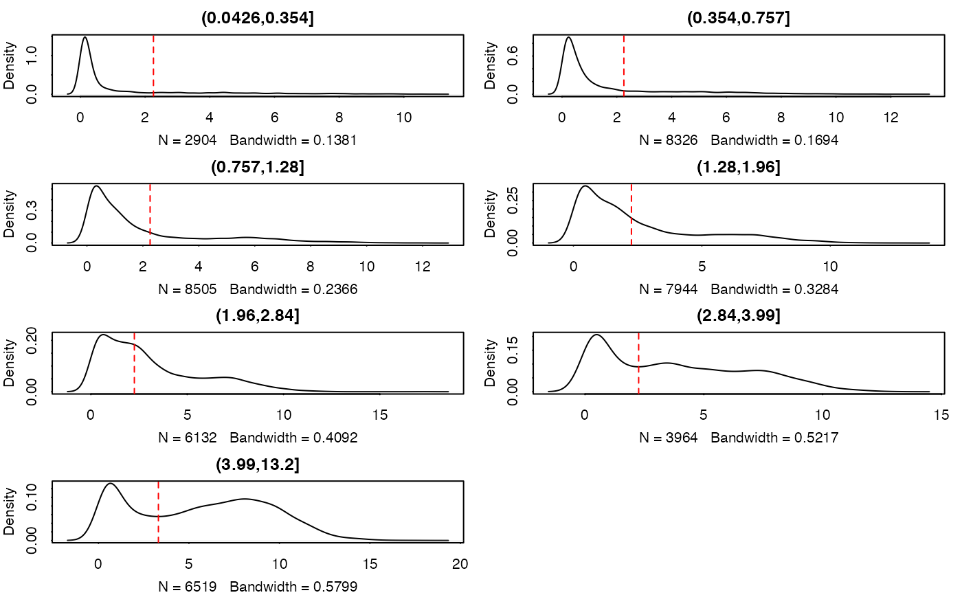
thresholdSCRNACountMatrix.RdAn adaptive threshold is calculated from the conditional mean of expression, based on 10 bins of the genes with similar expression levels. Thresholds are chosen by estimating cutpoints in the bimodal density estimates of the binned data. These density estimates currently exclude the zeros due to complications with how the bandwidth is selected. (If the bandwith is too small, then extra peaks/modes are found and everything goes haywire). If the diagnostic plots don't reveal any bimodal bins, this is probably the reason, and you may not need to threshold since background in the data are exact zeros.
thresholdSCRNACountMatrix(
  data_all,
  conditions = NULL,
  cutbins = NULL,
  nbins = 10,
  bin_by = "median",
  qt = 0.975,
  min_per_bin = 50,
  absolute_min = 0,
  data_log = TRUE,
  adj = 1
)
Arguments
- data_all
matrixof (possibly log-transformed) counts or TPM. Rows are genes and columns are cells.- conditions
Bins are be determined per gene and per condition. Typically contrasts of interest should be specified.
- cutbins
vectorof cut points.- nbins
integernumber of bins when cutbins is not specified.- bin_by
character"median", "proportion", "mean"- qt
when
bin_byis "quantile", what quantile should be used to form the bins- min_per_bin
minimum number of genes within a bin
- absolute_min
numericgiving a hard threshold below which everything is assumed to be noise- data_log
is
data_alllog+1 transformed? If so, it will be returned on the (log+1)-scale as well.- adj
bandwith adjustment, passed to
density
Value
list of thresholded counts (on natural scale), thresholds, bins, densities estimated on each bin, and the original data
Examples
data(maits,package='MAST', envir = environment())
sca <- FromMatrix(t(maits$expressionmat[,1:1000]), maits$cdat, maits$fdat[1:1000,])
#> Assuming data assay in position 1, with name et is log-transformed.
tt <- thresholdSCRNACountMatrix(assay(sca))
#> (0.0426,0.354]  (0.354,0.757]   (0.757,1.28]    (1.28,1.96]    (1.96,2.84]
#>       2.258200       2.258200       2.258200       2.258200       2.258200
#>    (2.84,3.99]    (3.99,13.2]
#>       2.258200       3.313588
tt <- thresholdSCRNACountMatrix(2^assay(sca)-1, data_log=FALSE)
#> (0.0426,0.354]  (0.354,0.757]   (0.757,1.28]    (1.28,1.96]    (1.96,2.84]
#>       2.258200       2.258200       2.258200       2.258200       2.258200
#>    (2.84,3.99]    (3.99,13.2]
#>       2.258200       3.313588
opar <- par(no.readonly = TRUE)
on.exit(par(opar))
par(mfrow=c(4,2))
plot(tt)
